For DataScientists: How to analyse multiple datasets
So you have gathered a load of data using the mindaffectBCI from yourself on different days, or from a group of people. Now you want to see if you can tweak the analysis settings to get much better performance in later days. As you know some machine learning, you know that tweaking the settings on a single dataset will just lead to overfitting. So you want to try new settings on all the data you have so far to see if your changes generalize to new data.
In this tutorial you will learn;
- How to load all the datasets in a directory
- And apply the standard mindaffectBCI classification pipeline to them, to generate a summary of the performance on all the datasets.
- How to tweak different settings to see if you can improve the general performance.
Note: in addition to using this notebook to analysis data gathered locally, you can perform analysis directly on-line on our Kaggle dataset or download this data for local off-line analysis.
Imports and configuration setup.
[ ]:
import numpy as np
from mindaffectBCI.decoder.datasets import get_dataset
import matplotlib.pyplot as plt
from mindaffectBCI.decoder.analyse_datasets import analyse_dataset, analyse_datasets, debug_test_dataset, debug_test_single_dataset
%matplotlib inline
%load_ext autoreload
%autoreload 2
Set the directory you want to load the datasets for analysis from
[ ]:
datasetsdir = "~/Desktop/datasets"
Check what datasets can be found in this directory
[ ]:
dataset_loader, dataset_files, dataroot = get_dataset('mindaffectBCI',exptdir=datasetsdir)
print("Got {} datasets\n{}".format(len(dataset_files),dataset_files))
Set the parameters for the analysis to run. Specificially:
test_idx: this is the trials to be used for performance evaluation in each dataset. All other trials are used for parameter estimation (in a nested cross-validation). Here we useslice(10,None)to say all trials after the 1st 10 are for testing.loader_args: dictionary of additional arguments to pass to theload_mindaffectBCI.pydataset loader, specifically the band-pass filter to usestopband=(5,25,'bandpass'), and the output sample rateout_fs=100.preprocessor_args: dictionary of additional arguments to pass to thepreprocess.pyoffline data pre-processor. Here we don’t specify any.model: the machine learning model to use. Here it’s the standardccamodel.clsfr_args: dictionary of additional arguments to pass to the model fitting proceduremodel_fitting.MultiCCA. Here we specify the brain event types to modelevtlabs=('re','fe')which means model the rising and falling edge responses only), the length of the brain responsetau_ms=450which means a response of 450 milliseconds, andrank=1to fix the model rank of 1.
As it runs this script will generate a lot of text and then a final summary plot. The key things to understand are:
- per-dataset decoding summary text. For each dataset a lot of summary info is generated saying things like the number of trials in the data-set, the preprocessing, the classifier parameter settings used etc. At the end of all this will be a block of text like this:
IntLen 69 138 190 260 329 381 450 520 \n Perr 1.00 0.57 0.43 0.19 0.14 0.05 0.05 0.05 AUDC 29.8 \n Perr(est) 0.87 0.49 0.48 0.11 0.07 0.07 0.05 0.03 PSAE 49.7 \n StopErr 1.00 1.00 1.00 0.60 0.43 0.33 0.33 0.33 AUSC 63.2 \n StopThresh(P) 0.93 0.93 0.93 0.58 0.38 0.33 0.33 0.33 SSAE 8.7 \n
This is a textual summary of the models performance as a decoding curve which says how a particular performance measure changes as the system gets increasing amounts of data within a single trial. Thus, this allows you to see how you would expect the system to perform if you manually stopped the trial after, say, 500 samples (which @100hz = 5 seconds). There are 4 key metrics reported here to assess the system performance.
* **Perr** : this is the probability of an error -- basically this says that over all of the training trials at each integeration-length if forced to stop what fraction of the trails would be incorrect.

* **Perr(est)** : in real usage the BCI doesn't actually know if it's prediction is wrong, but has to estimate it's confidence itself.  As these predictions are used to decide when to stop the trial, they should be as accurate as possible.  Perr(est) represents over all the test trails the systems own estimate of it's chance of being wrong with increasing integeration length.

* **StopErr** : The on-line system will Perr(est) to decide when to stop.  StopErr gives an estimate of how accurate this method of stopping a trial can be.  Due to trial-to-trial variation and accuracy of Perr(est) this can be better tha Perr (as the system can stop early on easy trials, but later on hard trials), or it can be much worse than Perr (if the estimates are very noisy so it stops at the wrong time.)   So this estimate should be as low as possible as early as possible.

* **StopThresh** : When making the StopErr results the system estimates a Perr(est) threshold which on-average stops at a given integeration length.  The StopThresh line gives these thresholds.   Ideally, this should be **exactly** equal the StopErr at every time point -- but if Perr(est) is incorrect or highly noisy it can be higher or lower than desired.   This gives a guide to how reliable Perr(est) stopping is for deciding when to stop a trial.

* **AUDC** : this is the Area Under the Decoding Curve, which is a single number -- lower better -- to characterise how fast and how low the Perr goes with time.

* **AUSC** : this is the Area Under the Stopping Curve, which is a similar single performance number for the stopping curve.
* **PSAE** and **SSAE** : are Summed Average Error for the Perr(est) estimates, and the StoppingThresholds.  Again lower is better for these.
- Dataset summary curve: After all the datasets have been run a final summary over all datasets will be generated, both as a textual summary like for the single trials. And as a datasets summary plot like this:
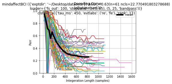
This plot shows for each dataset the summary Perr decoding curve, with the average over all datasets as the thick black line. Also in the title is a summary of the tested configuration and the cross datasets average AUDC to give an idea of the performance of this configuration over all the dataset.
[ ]:
analyse_datasets('mindaffectBCI',dataset_args=dict(exptdir=datasetsdir),
                 loader_args=dict(fs_out=100,stopband=((45,65),(5,25,'bandpass'))),
                 preprocess_args=None,
                 model='cca',test_idx=slice(10,None),clsfr_args=dict(tau_ms=450,evtlabs=('re','fe'),rank=1))
[ ]: